How to Create Pivot Table Charts and Pivot Chart Functions in Excel

excelcartstutorial.blogspot.com - pivot table chart or pivot chart is a chart feature of a pivot table for representing data. The function of a Pivot chart in Excel is to create a chart instantly via a pivot table. This feature can speed up the creation of graphs of data. Before creating a pivot chart in Excel you can read the previous tutorial on " How to Make a Pivot Table " for easy understanding.

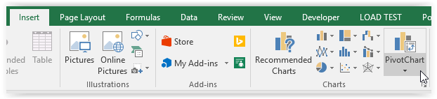
A. PivotChart Command Button in Excel

The Pivot Chart command button is located on the Insert ribbon in the Charts group section . The following is an illustration of the PivotChart command button ,

---

B. How to Make a Pivot Chart in Excel

Before creating a pivot table chart or pivot chart you need to create a pivot table from the data that will be created in the pivot chart .

Suppose we will use the example in the previous tutorial to create a paper mill sales chart from the following table,

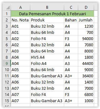
Note: Unique Note Number is obtained by each subscriber in a day.

A graph will be created showing the number of types of products in the 7 orders.

Here are the steps to create a pivot table chart,

1. Create a pivot table from data

   You can read the previous tutorial for creating a pivot table from the data above. So that the following results are obtained, bandarq online

   

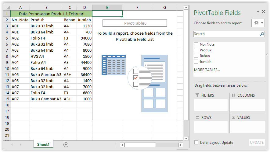
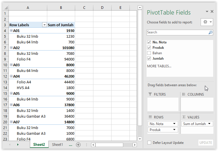
2. Set PivotTable Fields

   To set PivotTable Fields, adjust ROWS and COLUMN on Drag Fields . Suppose in this case you can (1) Checking No. Memorandum advance to make the data on a graph group, (2) Checking Product to charge members of the group, and (3) Checking the amount to give the value of the data on a graph.

   Here's an Illustration,

   

3. Create a Pivot Chart

   After creating the Pivot table, make sure you have selected (highlight) the table. Then click the PivotChart command button on the Insert ribbon .

   

4. Move the pivot table to a new sheet (optional)
   

   You can move the pivot table to a new sheet to display a chart without a pivot table on the sheet you are going to print.

   • Highlight the Pivot table

     

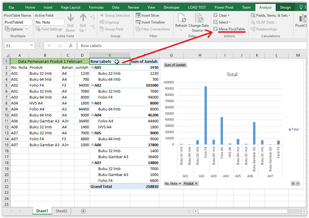
   • Click ribbon Analyze »Move Pivot Table
     

     So that the Move PivotTable window opens

   • Select New Worksheet

     

   • Click OK to move

     

5. Customize pivot data to add data and legends

   If you did step 4, then go back to the previous sheet and highlight the pivot chart to bring up the Field List in the Selection Pane . You can customize the data on the pivot chart by using the drag fields area.

   • Right click the graphic select Show Field List

     

   • Customize pivot data

     Suppose we will create a legend based on the type of product on the chart,